4 useful Google Sheets formatting tips

For many of us, Microsoft Excel is a tool we grew up using, which made it a natural candidate for any project involving numbers and formulas. Many electrical estimators in the industry either use Excel for estimating for the entirety of their estimating process, or for at least part of it, such as the output of their automated takeoffs, ready to assign costs. 

Today, with many of us working remotely, Microsoft’s online version of Excel has risen in popularity. However even with this cloud-based offering, many modern estimators prefer to use Google Sheets. As well as being free to use, Google Sheets is built “cloud-first”, giving it a slightly friendlier user experience. Yes it may be lacking some of the more complex capabilities needed if you’re using hundreds of millions of cells (as opposed to Sheets’ five-million cell limit) but for basic to mid-tier users, it’s a robust and free solution. 

Whether you’ve always been a Google Sheets fan, or you’ve recently made the switch, it’s worth learning a few formatting tips to increase your efficiency. 

Here, we’ll take you through four handy tips every Google Sheets user should know.

4 useful Google Sheets formatting tips

1. Conditional formatting in Google Sheets

While the name “Conditional formatting” may sound like a dark art, Conditional formatting is the method that helps you to achieve these handy use cases:

• Turn a cell a certain colour if a condition is met (for example a “YES” response is entered and the cell turns green to let you know that task is complete)
• To let you know if you’ve entered the same value twice (if duplicate data would be incorrect for your project)
• To alert you to the fact a cell is empty (if indeed it’s meant to be filled)

Here are the steps of how to use conditional formatting to set up your Google Sheet for any of the options above.

Select your cells

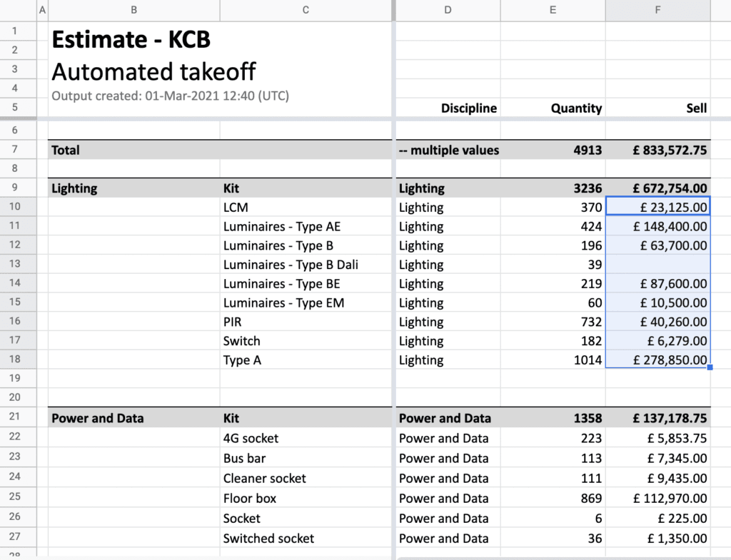
Within your sheet highlight the list of cells you’d like to include in the rule. In this instance, we’re using all of the cells within column “F” of our estimating spreadsheet.

Select “Format” and “Conditional Formatting” from the top bar

Next, choose the Conditional Formatting option under the “Format” tab.

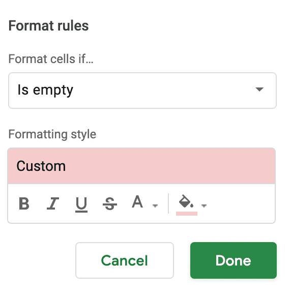
Select your trigger

Here you’ll need to choose the “if this then that” trigger that will cause your cell to change its format. Here, we want the cell to turn red if it’s empty (so we can check if something has been missed within the estimate). Under “Format rules” we’ll select “Format cells if is empty” as the trigger.

Choose the formatting style

Next we’ll need to choose the formatting style. Here you can choose one of the preset styles (we’re using a red background as an alert style message), or you can create your own format using “Custom format”.

Select “Done”

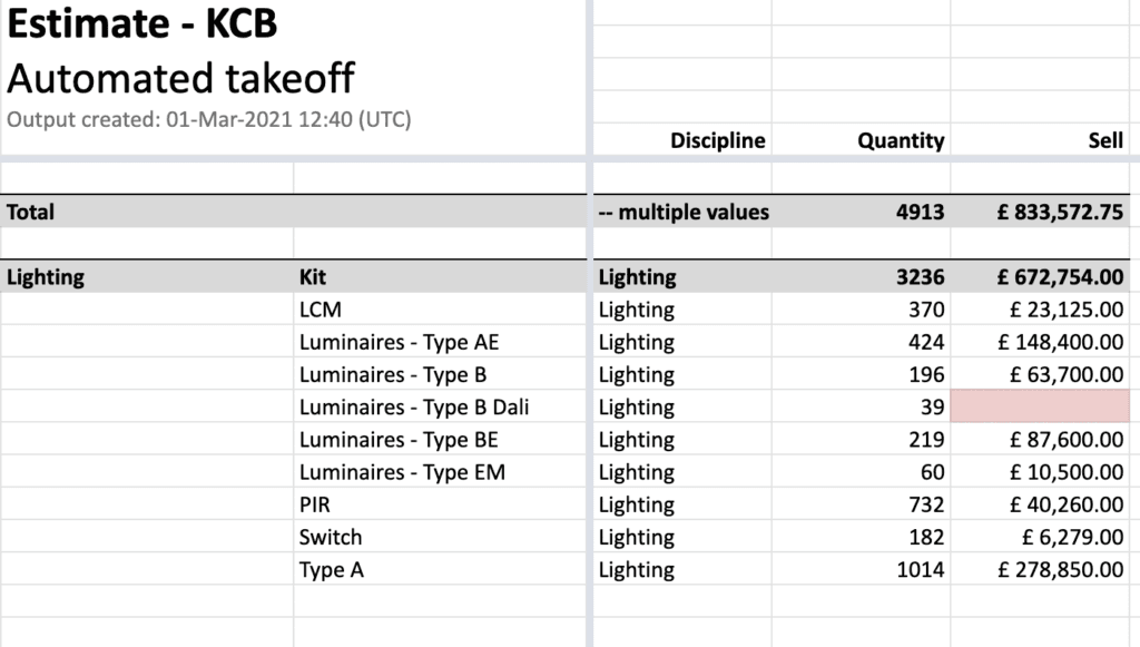
Once the formatting is set up click “Done” and you can automatically see on the estimating sheet the cells turning red that are empty. In some instances this will be fine as no information is needed, however in others it allows me to return to my estimate and see where the information has been missed, or to re-add this to my takeoff tool to submit a new count (something which can handily be done by reprocessing the project in Countfire). 

Once you know how to do one type of Conditional formatting the others are just as simple. Change the trigger and the formatting option and you can automate plenty of checks and formats to your Sheet without any manual work. 

2. Google Sheets formatting shortcuts

At Countfire we’re a big fan of keyboard shortcuts. We even have pages within our company wiki, dedicated to helping our team to learn shortcuts that will save them time in programs we use within the company. 

In Google Sheets the same is true. Shortcuts help you to work faster and without need of your mouse in many cases. Here are the most used Google Sheets shortcuts to get you started:

Select column

• Ctrl + Space (Mac & PC)

Select row

• Shift + Space (Mac - and if you’re not sure what “Shift” is on Mac, it’s the arrow pointing upwards below caps lock)
• Shift + Space (PC)

Insert link

• Command + k (Mac)
• Ctrl + k (PC)

Format as a decimal 

• Ctrl + Shift + 1 (Mac & PC)

Move to beginning of the row

• Fn + left arrow (Mac)
• Home (PC)

Move to end of the row

• Fn + right arrow (Mac)
• End (PC)

If you’ve already committed these basic shortcuts to memory, there are always plenty more to learn. Check out this guide for the full list.

3. Copy and paste formulas

There are many reasons you may want to copy and paste formulas from one cell to another. A few reasons we can think of would be to save you having to format each individual cell, and to ensure consistency. For example, if one of your cells has a two-point decimal number but the rest only have a one-point number, it’s going to feel inconsistent and won’t be easily scannable. Here’s how to tighten up the formatting:

Copy using the Paint format tool

To copy over a formula, first select the cell which has the correct formula applied. Then select “Paint format” by using the paint roller icon as shown here:

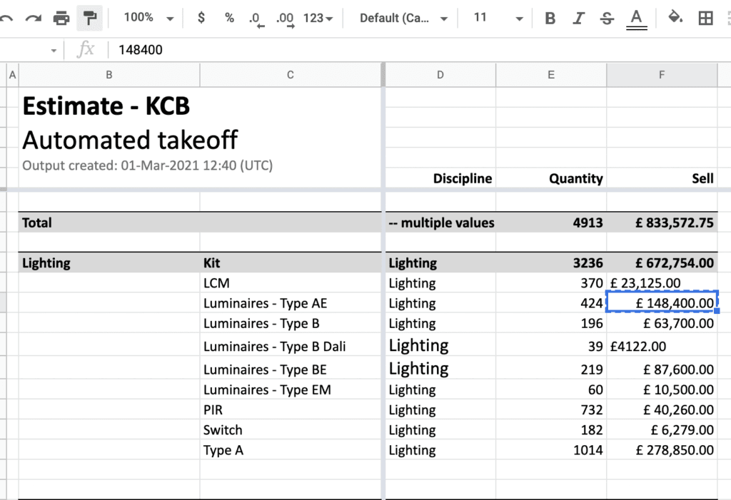
Select the cell you want to copy the formula into

Now simply click on the cell you want to copy the formula to. You’ll see the cell changes automatically to the same format as the one previously. You can also use the paint formula tool across multiple cells at once and it will pick up any outliers and add them into the same format.

4. Text formatting

Thanks to badly formatted PDF drawings, or just a hastily inputted project, sometimes your Google Sheet can require some housekeeping to make it “client ready”. If one of the issues is that text has been added that’s not in a consistent format (i.e. all uppercase, all lowercase or what Sheets calls “Proper Case” which means the first letter of each word is capitalised) you can rectify this using the below method:

Find an empty cell and create your formula

Move your cursor into an empty cell and then write one of the below formulas, followed by the cell that you’d like to change to upper, lower or proper case style.

=upper(c1)

=lower(c1)

=proper(c1)

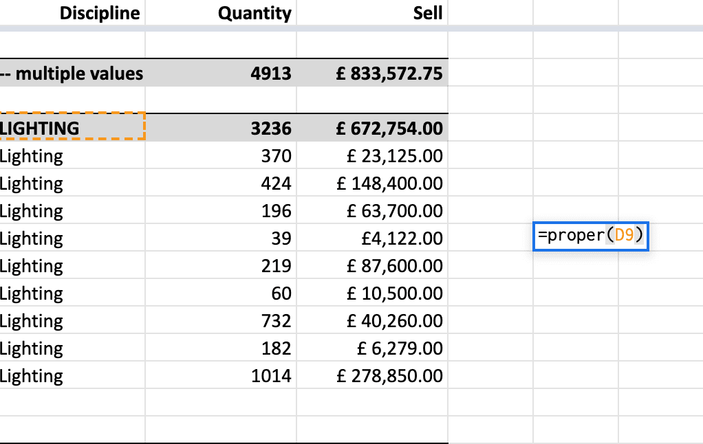
Select enter once written and you’ll see your original cell has been copied but is now in the correct format. 

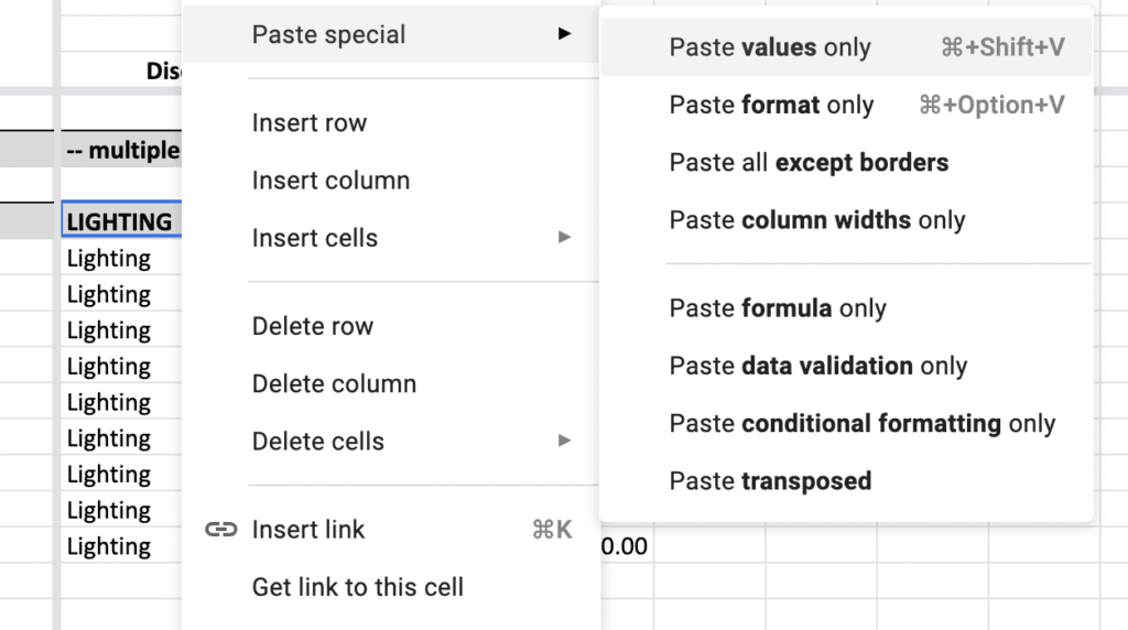
Copy your formula (value only)

Select the cell where your copy is now written in the correct format and select “Copy”. Then move to the original cell where you wish to change the text, right-click and choose “Paste special > Paste values only”. Here, you should see that your cell has now been copied into the correct format.

Of course, this is great for one or two cells but for changing the format of a list of cells, it could take a considerable amount of time. In this instance, you may want to install what Google Sheets calls an “Add-on”.

Select the Add-ons tab in the top bar and select “Get add-ons”. If you cannot see the Add-ons tab it’s likely you either don’t have permission to edit that Google Sheet, or this is a setting which has been applied by your administrator.

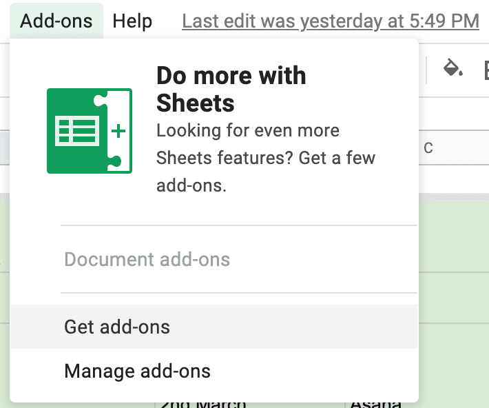
Once you have the ability to install an Add-on you can then start using something such as ChangeCase which will allow you to change mass amounts of cells all in one hit, saving a lot of time. 

Final thoughts

While Google Sheets formatting can seem complex on first glance, the short-term pain is worth it in the long-term gain of increased efficiency and productivity. By learning a few simple tips and tricks, you can work smarter and get more estimates in on time.